Why Does PCA Work? A Geometric and Statistical Derivation

Principal Component Analysis (PCA) is one of the most widely used methods for dimensionality reduction. It appears in exploratory data analysis, visualization, noise reduction, and machine learning pipelines.

But why does it work?

PCA does not simply select a few original features. Instead, it constructs new, mutually orthogonal directions that capture as much of the data’s variation as possible. These directions turn out to be the eigenvectors of the covariance matrix, ordered by their corresponding eigenvalues.

This article derives that result from first principles. We will connect three perspectives:

1. Statistical: Find directions that preserve the greatest variance.
2. Geometric: Project data onto a lower-dimensional subspace while losing as little as possible.
3. Computational: Use eigendecomposition or Singular Value Decomposition (SVD) to find the optimal subspace.

Finally, we will test these connections on a reproducible synthetic dataset with 50 features.

1. The problem: representing high-dimensional data

Suppose our dataset contains $n$ observations and $p$ numerical features. We represent it as a matrix:

$$X \in \mathbb{R}^{n \times p}.$$

Each row represents an observation, and each column represents a feature.

When $p$ is large, analyzing the dataset directly can be difficult. We may want a lower-dimensional representation with only $k$ dimensions, where $k < p$.

A simple approach would be to select $k$ of the original features. However, this can discard important relationships between features. A better alternative is to construct new features as linear combinations of the original ones.

Before doing so, we center the data by subtracting the mean of each feature:

$$X_c = X - \mathbf{1}\mu^\top,$$

where $\mu \in \mathbb{R}^{p}$ contains the feature means and $\mathbf{1}$ is a vector of $n$ ones.

After centering, each feature has mean zero, up to numerical precision. The sample covariance matrix is then

$$S = \frac{1}{n-1}X_c^\top X_c.$$

The matrix $S \in \mathbb{R}^{p \times p}$ summarizes the variances of individual features and the covariances between pairs of features.

Our goal is to discover a small number of directions that retain as much useful variation in the centered data as possible.

2. Why maximize projected variance?

Consider a single direction $w \in \mathbb{R}^{p}$. Projecting each observation onto this direction produces a one-dimensional representation:

$$z = X_cw.$$

Here, $z \in \mathbb{R}^{n}$ contains the projected values for all observations.

The sample variance of these projected values is

$$\operatorname{Var}(z) = \frac{1}{n-1}z^\top z.$$

Substituting $z = X_cw$, we obtain

$$\begin{aligned} \operatorname{Var}(z) &= \frac{1}{n-1}(X_cw)^\top(X_cw)\\ &= \frac{1}{n-1}w^\top X_c^\top X_cw\\ &= w^\top Sw. \end{aligned}$$

Therefore, the variance captured by a direction is determined by the quadratic form $w^\top Sw$.

There is one complication: multiplying $w$ by a large constant also multiplies the projected variance by the square of that constant. Without a constraint, we could increase the objective indefinitely without finding a more meaningful direction.

We solve this by requiring the direction to have unit length:

$$w^\top w = 1.$$

Our optimization problem becomes

$$\boxed{ \begin{aligned} \max_w \quad & w^\top Sw\\ \text{subject to} \quad & w^\top w = 1. \end{aligned} }$$

This is the central idea behind PCA: find a unit direction along which the projected data has maximum variance.

The statistical formulation of PCA is associated with the work of Hotelling, while the broader geometric perspective of fitting lower-dimensional linear structures has earlier roots in Pearson’s work.(Hotelling (1933), Pearson (1901), and Jolliffe and Cadima (2016))

3. Deriving the first principal component

We now solve the optimization problem.

3.1 Use a Lagrange multiplier

We want to maximize $w^\top Sw$ subject to $w^\top w=1$. Introduce a Lagrange multiplier $\lambda$ and define

$$\mathcal{L}(w,\lambda) = w^\top Sw-\lambda(w^\top w-1).$$

Taking the gradient with respect to $w$ gives

$$\nabla_w \mathcal{L} = 2Sw-2\lambda w.$$

At a stationary point, the gradient must equal zero:

$$2Sw-2\lambda w=0.$$

Rearranging yields

$$\boxed{Sw=\lambda w.}$$

This is precisely the eigenvector equation.

The direction $w$ must be an eigenvector of the covariance matrix, and $\lambda$ is its associated eigenvalue.

3.2 Why choose the largest eigenvalue?

The eigenvector equation tells us which directions are candidates, but we still need to determine which candidate maximizes the variance.

Multiplying $Sw=\lambda w$ on the left by $w^\top$ gives

$$w^\top Sw = \lambda w^\top w.$$

Since $w^\top w=1$,

$$\boxed{w^\top Sw=\lambda.}$$

The variance captured by a unit eigenvector is therefore equal to its eigenvalue.

Because the covariance matrix is symmetric and positive semidefinite, its eigenvalues are real and nonnegative. Let them be ordered as

$$\lambda_1 \geq \lambda_2 \geq \cdots \geq \lambda_p \geq 0.$$

The maximum attainable variance is $\lambda_1$. Consequently, the first principal component is an eigenvector associated with the largest eigenvalue:

$$Sw_1=\lambda_1w_1.$$

Its projected data is $X_cw_1$, and its variance is $\lambda_1$.

Two details are worth remembering:

• The sign of an eigenvector is arbitrary. The directions $w_1$ and $-w_1$ describe the same one-dimensional subspace and preserve identical variance.
• If the largest eigenvalue is repeated, there may be multiple equally optimal directions. The individual first principal component is then not unique, although its optimal subspace is well defined up to the corresponding eigenspace.

The key result: The first principal component is a leading covariance eigenvector because maximizing projected variance under a unit-length constraint leads directly to the eigenvector equation.

4. From one component to $k$ components

Keeping one dimension may discard too much information. We therefore extend the problem to a $k$-dimensional subspace.

Let

$$V_k = \begin{bmatrix} w_1 & w_2 & \cdots & w_k \end{bmatrix} \in \mathbb{R}^{p \times k},$$

where the columns are orthonormal:

$$V_k^\top V_k=I_k.$$

The lower-dimensional representation is

$$Z=X_cV_k.$$

Its total sample variance, summed across the $k$ orthogonal component directions, is

$$\begin{aligned} \operatorname{Var}_{\text{total}}(Z) &= \frac{1}{n-1}\|X_cV_k\|_F^2\\ &= \operatorname{tr}(V_k^\top S V_k). \end{aligned}$$

Here, $\|\cdot\|_F$ denotes the Frobenius norm, and $\operatorname{tr}(\cdot)$ denotes the matrix trace.

We now want to maximize

$$\boxed{ \max_{V_k^\top V_k=I_k} \operatorname{tr}(V_k^\top S V_k). }$$

The solution is a subspace spanned by eigenvectors corresponding to the $k$ largest eigenvalues of $S$. Its maximum retained variance is

$$\boxed{\sum_{j=1}^{k}\lambda_j.}$$

This result follows from the maximum principle for sums of eigenvalues, commonly associated with Ky Fan’s work. It extends the one-component argument: rather than retaining just the direction with the greatest variance, we retain the $k$-dimensional subspace with the greatest total variance. (Fan (1951))

4.1 Explained variance

The total variance of the centered dataset is

$$\operatorname{tr}(S)=\sum_{j=1}^{p}\lambda_j.$$

The proportion of variance retained by the first $k$ components is therefore

$$\boxed{ \operatorname{EVR}(k) = \frac{\sum_{j=1}^{k}\lambda_j} {\sum_{j=1}^{p}\lambda_j}. }$$

This is called the cumulative explained variance ratio.

For example, if the first five components explain 90% of the total variance, then retaining those components preserves 90% of the dataset’s variance under this measure.

It does not mean that 90% of every feature, every observation, or every task-relevant signal has been preserved. Explained variance is a specific mathematical criterion, not a universal measure of information.

5. The geometric connection: minimizing reconstruction error

Variance maximization gives us one reason to use PCA. There is another, geometric interpretation: PCA finds the best lower-dimensional linear subspace for reconstructing centered data under squared Euclidean error.

Suppose we project the observations into the subspace spanned by $V_k$:

$$Z=X_cV_k.$$

We can reconstruct an approximation in the original feature space by projecting back:

$$\hat X_c=ZV_k^\top=X_cV_kV_k^\top.$$

The reconstruction residual is

$$R=X_c-\hat X_c =X_c(I-V_kV_k^\top).$$

A natural measure of reconstruction quality is the sum of squared errors:

$$E(V_k)=\|X_c-\hat X_c\|_F^2.$$

Because $V_kV_k^\top$ is an orthogonal projection matrix, the squared norm separates into the energy retained by the projection and the energy discarded by it. Thus,

$$\begin{aligned} E(V_k) &=\|X_c\|_F^2-\|X_cV_k\|_F^2\\ &=\|X_c\|_F^2 -\operatorname{tr}(V_k^\top X_c^\top X_cV_k). \end{aligned}$$

Using $X_c^\top X_c=(n-1)S$, we get

$$\boxed{ E(V_k) =(n-1)\left[ \operatorname{tr}(S) -\operatorname{tr}(V_k^\top SV_k) \right]. }$$

Notice that $\operatorname{tr}(S)$ is constant for a fixed dataset. Minimizing the reconstruction error is therefore equivalent to maximizing the variance retained by the projection.

This establishes the connection:

$$\boxed{ \begin{gathered} \text{Maximum retained variance}\\ \Updownarrow\\ \text{Minimum squared reconstruction error} \end{gathered} }$$

Both objectives select the subspace spanned by the leading covariance eigenvectors.

This is a precise statement about centered data, orthogonal linear projections, and squared reconstruction error. It does not claim that PCA minimizes every possible loss function or preserves all information relevant to a downstream task.

The geometric interpretation is closely connected to Pearson’s early work on lines and planes of closest fit. The matrix approximation perspective is formalized by the Eckart–Young theorem.(Pearson (1901) and Eckart and Young (1936))

5.1 The SVD connection

There is a computationally useful way to express the same result.

Take the Singular Value Decomposition of the centered data matrix:

$$X_c=U\Sigma W^\top.$$

The columns of $W$ are the right singular vectors, and the diagonal entries of $\Sigma$ are the singular values:

$$\sigma_1\geq \sigma_2\geq\cdots\geq 0.$$

Since

$$S=\frac{1}{n-1}X_c^\top X_c,$$

substituting the SVD gives

$$S=\frac{1}{n-1}W\Sigma^\top\Sigma W^\top.$$

Therefore, the covariance eigenvectors are the right singular vectors of $X_c$, and their eigenvalues satisfy

$$\boxed{\lambda_j=\frac{\sigma_j^2}{n-1}.}$$

The optimal rank-$k$ reconstruction error is consequently

$$\boxed{ E_k=\sum_{j>k}\sigma_j^2 =(n-1)\sum_{j>k}\lambda_j. }$$

This is the low-rank approximation connection: keeping the leading $k$ singular directions minimizes the squared Frobenius reconstruction error among rank-$k$ approximations.

In practice, PCA can be computed through covariance eigendecomposition or directly through SVD. Direct SVD is often numerically preferable when forming the covariance matrix could amplify conditioning problems. Which method is faster depends on the relative sizes of $n$ and $p$, the implementation, and the computational environment. (Eckart and Young (1936); see also the scikit-learn PCA documentation)

6. Numerical verification: a 50-dimensional experiment

The derivation tells us what PCA should do. We can now test its consequences on a controlled dataset.

Rather than using a two-dimensional example that can be inspected visually, we construct a dataset with 2,000 observations and 50 features.

6.1 Constructing the dataset

We generate five latent factors and let each factor influence a block of ten observed features. Independent Gaussian noise is then added to the observations.

A simplified representation of the data-generating process is

$$X=ZA^\top+E,$$

where:

• $Z\in\mathbb{R}^{2000\times5}$ contains the latent factor values.
• $A\in\mathbb{R}^{50\times5}$ contains the feature loadings.
• $E\in\mathbb{R}^{2000\times50}$ contains independent Gaussian noise.

We use a fixed random seed for reproducibility, set the noise standard deviation to 0.35, and center the generated data before performing PCA.

This setup provides two things to investigate: whether PCA recovers the planted five-dimensional factor subspace, and whether its reconstruction error is lower than that of randomly chosen subspaces.

6.2 Inspecting the correlation structure

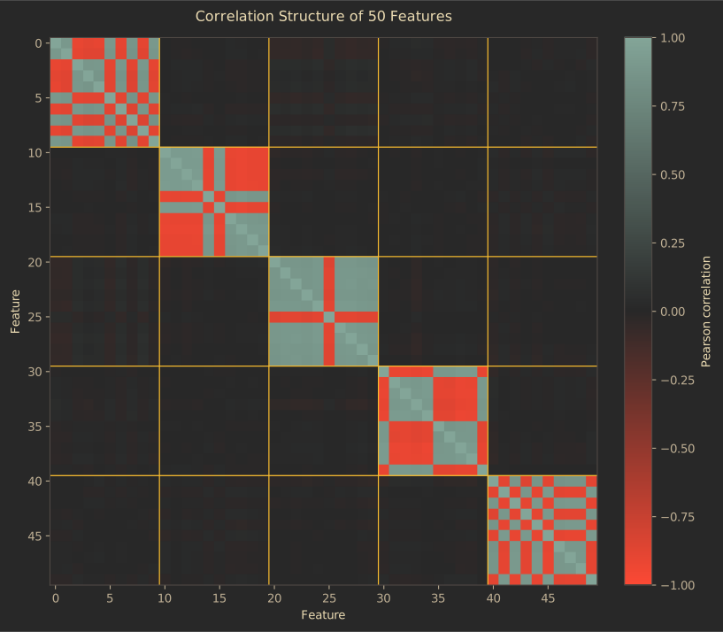
Figure 1. Feature correlation structure of the synthetic dataset. The block structure reflects the way the latent factors influence groups of features.

The visible block structure is a consequence of the data-generation process. Features influenced by the same latent factor tend to share variation.

This does not mean that real datasets necessarily have clean blocks or five underlying factors. Here, the controlled structure gives us a known reference against which to evaluate PCA.

6.3 Measuring explained variance

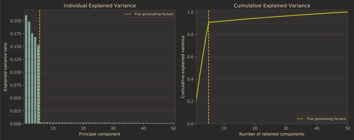
Figure 2. Cumulative explained variance as the number of retained principal components increases.

Our experiment produced the following results:

Components retained	Cumulative variance retained
1	21.07%
2	40.90%
3	58.51%
5	90.69%
10	91.98%
20	94.33%
30	96.45%
40	98.35%
50	100.00%

The first five principal components retain approximately 90.69% of the total variance. Retaining all 50 components preserves 100% of the variance, apart from negligible floating-point effects.

Why do five components not explain exactly 100% of the variance, given that we generated five latent factors?

Because the observed dataset also contains noise. The noise contributes additional variation outside the planted latent subspace. The five-factor construction does not imply that the observed matrix has rank five.

The result illustrates an important distinction: the number of latent factors used to generate data is not automatically the number of principal components required to explain all observed variance.

6.4 Comparing PCA with random subspaces

To test the geometric interpretation, we compare PCA against 50 randomly generated orthogonal subspaces at each selected dimension.

For each $k$, we calculate the squared reconstruction error and express it as a percentage of the total squared norm of the centered dataset.

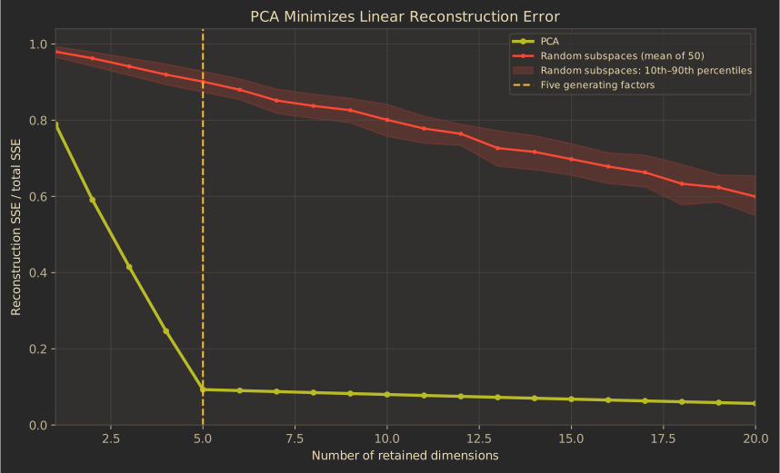
Figure 3. Normalized reconstruction error for PCA and sampled random subspaces. PCA gives the minimum error theoretically; the random-subspace results illustrate this behavior empirically.

For five components, PCA retains 90.69% of the variance and discards 9.31%. Its normalized reconstruction error is therefore approximately 9.31%.

The mean normalized error across the 50 sampled random five-dimensional subspaces is approximately 90.12%.

Components $k$	PCA error	Mean random-subspace error
1	78.93%	97.99%
2	59.10%	96.25%
3	41.49%	94.12%
5	9.31%	90.12%
10	8.02%	80.08%
20	5.67%	59.95%

In this experiment, PCA’s reconstruction error was no greater than that of any sampled random subspace for the tested dimensions.

That is consistent with the theoretical result, but the random comparison is illustrative rather than a proof. Sampling 50 alternatives cannot establish optimality over every possible subspace. The proof comes from the variance-maximization and low-rank approximation results derived earlier.

6.5 Checking the numerical identities

We also verify the mathematical identities directly.

Check 1: covariance eigenvalues versus singular values.

We compare the eigenvalues of the sample covariance matrix with the squared singular values divided by $n-1$:

$$\lambda_j\stackrel{?}{=}\frac{\sigma_j^2}{n-1}.$$

The maximum absolute difference in our run was approximately $1.60\times10^{-14}$, consistent with floating-point numerical precision.

Check 2: reconstruction error versus the discarded singular-value tail.

For each tested $k$, we compare the directly computed reconstruction error with

$$E_k\stackrel{?}{=}\sum_{j>k}\sigma_j^2.$$

The values agreed to numerical precision for all tested dimensions.

Check 3: recovery of the planted factor subspace.

We compare the five-dimensional subspace spanned by the leading principal components with the planted factor subspace. The largest principal angle between the two subspaces was approximately $1.26^\circ$, and the Frobenius norm of the difference between their projection matrices was approximately 0.0544.

These results indicate close recovery of the planted subspace in this controlled experiment. The principal angles compare the subspaces as wholes; they do not require individual PCA directions to correspond one-to-one with the original latent factors.

Together, the checks provide numerical evidence that the implementation is consistent with the theoretical relationships.

7. What PCA does not guarantee

PCA has a strong mathematical foundation, but its assumptions and objective matter.

7.1 Centering is not standardization

Centering subtracts each feature’s mean. Standardization additionally scales features, often to unit variance.

If one feature is measured in thousands and another in fractions, the high-magnitude feature may dominate the covariance matrix. Whether to standardize depends on the meaning of the features and the analytical objective; it is not automatically necessary in every application.

7.2 High variance is not always useful information

PCA preserves variation, not necessarily predictive value. A low-variance feature can be essential for predicting a target, while a high-variance feature can mostly represent irrelevant fluctuations.

Consequently, retaining a large explained-variance percentage does not guarantee strong predictive performance.

7.3 Outliers can change the components

Covariance and variance are sensitive to extreme observations. A small number of outliers can substantially alter the leading principal directions.

Data inspection and, when appropriate, robust alternatives should be considered before interpreting the components.

7.4 PCA is a linear method

PCA finds an optimal linear subspace under its objective. It does not necessarily discover nonlinear structure.

A dataset may lie near a curved manifold that cannot be represented well by a low-dimensional linear projection. In such cases, other dimensionality-reduction approaches may be more appropriate, depending on the task.

7.5 Explained variance is not a universal stopping rule

Choosing $k$ by a threshold such as 90% or 95% is a useful heuristic, not a mathematical guarantee of downstream usefulness. The choice should also reflect interpretability, computational requirements, reconstruction quality, and—when applicable—performance on held-out data.

For practical implementation details and solver considerations, consult the scikit-learn PCA documentation.

8. Conclusion

PCA works because several mathematical ideas converge on the same solution.

First, maximizing the variance of a unit projection leads to the eigenvector equation for the covariance matrix. The largest eigenvalue identifies the direction with the greatest projected variance.

Second, extending the problem to $k$ orthogonal directions shows that the leading $k$ eigenvectors maximize total retained variance.

Third, projecting onto this subspace minimizes squared reconstruction error among $k$-dimensional orthogonal linear projections of the centered data. The SVD expresses the same result through the singular values and gives a direct formula for the discarded reconstruction error.

The numerical experiment supports these connections: the covariance eigenvalues agree with the SVD relationship, the reconstruction error agrees with the discarded singular-value tail, and PCA closely recovers the planted factor subspace.

The broader lesson is that PCA is not merely a convenient transformation. Its usefulness follows from a precise optimization objective. Understanding that objective also tells us when PCA is appropriate—and when preserving variance may not be enough.

References

1. Pearson, K. (1901). LIII. On lines and planes of closest fit to systems of points in space. The London, Edinburgh, and Dublin Philosophical Magazine and Journal of Science, 2(11), 559–572.

2. Hotelling, H. (1933). Analysis of a complex of statistical variables into principal components. Journal of Educational Psychology, 24(6), 417–441.

3. Jolliffe, I. T., & Cadima, J. (2016). Principal component analysis: a review and recent developments. Philosophical Transactions of the Royal Society A: Mathematical, Physical and Engineering Sciences, 374(2065), 20150202.

4. Eckart, C., & Young, G. (1936). The approximation of one matrix by another of lower rank. Psychometrika, 1, 211–218.

5. Fan, K. (1951). Maximum properties and inequalities for the eigenvalues of completely continuous operators. Proceedings of the National Academy of Sciences, 37(11), 760–766.

6. scikit-learn developers. PCA: Principal component analysis. scikit-learn documentation.