Eigenvectors: From Linear Transformations to Principal Component Analysis

Eigenvectors are among the most useful mathematical objects in data science. They appear in linear algebra, differential equations, graph algorithms, dynamical systems, and machine learning. Yet their importance is not merely that they simplify matrix calculations. They help us identify directions along which a transformation has a particularly simple effect.

Principal Component Analysis (PCA) uses precisely this idea to understand the geometry of data. By finding the eigenvectors of a covariance matrix, PCA identifies directions of maximum variance and constructs a lower-dimensional representation of the observations.

This connection is worth understanding from first principles. Rather than treating PCA as an algorithm that happens to return principal components, we will derive why eigenvectors appear, examine a higher-dimensional transformation, and follow the mathematics from covariance to projection.

1. Eigenvectors: Directions a transformation preserves

Consider a linear transformation represented by a square matrix $A$. Given a vector $v$, the transformation produces a new vector:

$$Av.$$

In general, the resulting vector may differ from the original in both magnitude and direction. However, some nonzero vectors have a special property: applying the transformation changes their magnitude without moving them away from their original line.

These vectors are called eigenvectors.

A nonzero vector $v$ is an eigenvector of $A$ if

$$\boxed{Av=\lambda v}$$

for some scalar $\lambda$, called the eigenvalue associated with $v$.

The equation says that the transformation’s effect on $v$ is equivalent to multiplying it by a scalar.

• If $\lambda>1$, the vector’s magnitude increases.
• If $0<\lambda<1$, its magnitude decreases.
• If $\lambda<0$, its orientation reverses as well as scaling.
• If $\lambda=0$, the vector is mapped to the zero vector.

The eigenvector itself is not unique: if $v$ is an eigenvector, then any nonzero scalar multiple $cv$ is also an eigenvector associated with the same eigenvalue.

Finding eigenvalues

Starting with

$$Av=\lambda v,$$

we rearrange the equation:

$$(A-\lambda I)v=0,$$

where $I$ is the identity matrix.

For a nonzero solution $v$ to exist, the matrix $A-\lambda I$ must be singular. Therefore, the eigenvalues satisfy the characteristic equation

$$\boxed{\det(A- \lambda I)=0}.$$

Once an eigenvalue is known, we solve

$$(A- \lambda I)v=0$$

to obtain its corresponding eigenvectors.

For small matrices, we can often do this by hand. For larger matrices, numerical algorithms are more practical. But the underlying definition remains the same, regardless of matrix size.

2. A four-dimensional linear transformation

A two-dimensional example is convenient for drawing arrows, but it can hide an important point: eigenvectors are not inherently two-dimensional. The same mathematical principle applies in any finite-dimensional vector space.

Let us consider a symmetric matrix $A\in\mathbb{R}^{4\times4}$. We construct it using an orthogonal matrix $Q$ and a diagonal matrix of distinct eigenvalues:

$$A=Q\Lambda Q^\top,$$

where

$$\Lambda= \begin{bmatrix} 7&0&0&0\\ 0&4&0&0\\ 0&0&2&0\\ 0&0&0&0.5 \end{bmatrix}, \qquad Q^\top Q=I.$$

The columns of $Q$, denoted by $v_1,\ldots,v_4$, are orthonormal eigenvectors. Because $Q$ is orthogonal,

$$AQ=Q\Lambda.$$

Reading this equation column by column gives

$$Av_i=\lambda_i v_i, \qquad i=1,\ldots,4.$$

The four eigenvalues are $7$, $4$, $2$, and $0.5$. The transformation therefore acts differently along four mutually orthogonal directions.

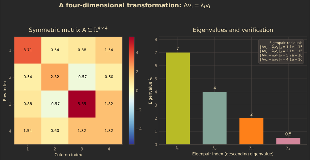
Figure 1. A four-dimensional transformation represented by its matrix and eigenvalues. The residuals verify numerically that the computed eigenpairs satisfy the defining equation.

The matrix heatmap makes the transformation’s entries visible, while the eigenvalue plot summarizes its action along the eigenvector directions. The numerical residuals are

$$r_i=\|Av_i-\lambda_i v_i\|_2.$$

In exact arithmetic, every residual would be zero. In floating-point computation, values close to machine precision indicate that the calculated eigenpairs satisfy the equation to numerical accuracy.

Notice what this example does not establish: the eigenvalues are not variances merely because they are eigenvalues. They describe scaling under this particular transformation. Their interpretation depends on the matrix being analyzed.

That distinction becomes essential when we move to PCA.

3. From observations to a covariance matrix

Suppose a dataset contains $n$ observations and $p$ numerical features. Arrange it into a matrix

$$X\in\mathbb{R}^{n\times p},$$

where rows represent observations and columns represent features.

Each observation is a point in a $p$-dimensional feature space. When $p$ is large, visualizing the complete dataset becomes difficult. We would like to find a smaller set of directions that preserves as much useful information as possible.

PCA begins by centering the data. Let the mean of feature $j$ be

$$\mu_j=\frac{1}{n}\sum_{i=1}^{n}X_{ij}.$$

Subtract each feature’s mean from its observations to obtain the centered data matrix:

$$X_c=X-\mathbf{1}\mu^\top,$$

where $\mathbf{1}$ is an $n$-dimensional vector of ones and $\mu$ contains the feature means.

The sample covariance matrix is then

$$\boxed{S=\frac{1}{n-1}X_c^\top X_c}.$$

This is a $p\times p$ matrix. Its diagonal entries are feature variances, and its off-diagonal entries are covariances between pairs of features.

Two properties are especially important:

1. Symmetry: $S^\top=S$.

2. Positive semidefiniteness: for every vector $w$,

   $$w^\top Sw =\frac{1}{n-1}\|X_cw\|_2^2 \geq 0.$$

Consequently, all eigenvalues of $S$ are real and nonnegative. Its eigenvectors can be chosen to form an orthonormal basis.

These are not arbitrary mathematical conveniences. They are the properties that make covariance-based PCA well behaved.

4. Why maximizing variance leads to eigenvectors

Now comes the central derivation.

Suppose we want to represent every centered observation using one direction $w$, where $w\in\mathbb{R}^{p}$ and $\|w\|_2=1$.

The scalar projection of observation $x_i$ onto this direction is

$$z_i=x_i^\top w.$$

For all observations together, the projected values form the vector

$$z=X_cw.$$

Because the original features have been centered, the projected values are also centered. Their sample variance is therefore

$$\begin{aligned} \operatorname{Var}(z) &=\frac{1}{n-1}z^\top z\\ &=\frac{1}{n-1}(X_cw)^\top(X_cw)\\ &=w^\top \left(\frac{1}{n-1}X_c^\top X_c\right)w\\ &=\boxed{w^\top Sw}. \end{aligned}$$

Thus, finding the direction with maximum projected variance becomes the optimization problem

$$\boxed{ \begin{aligned} \max_w\quad & w^\top Sw\\ \text{subject to}\quad & w^\top w=1. \end{aligned} }$$

Why do we need the unit-length constraint? Without it, multiplying $w$ by an arbitrarily large constant would increase the objective indefinitely. The constraint makes us compare directions rather than arbitrary vector magnitudes.

Deriving the eigenvalue equation

We can solve this constrained optimization problem using a Lagrange multiplier $\lambda$:

$$\mathcal{L}(w,\lambda) =w^\top Sw-\lambda(w^\top w-1).$$

Differentiating with respect to $w$ and setting the gradient to zero gives

$$\nabla_w\mathcal{L}=2Sw-2\lambda w=0.$$

Rearranging,

$$\boxed{Sw=\lambda w}.$$

This is the eigenvalue equation.

The result is the key connection: the stationary directions of projected variance are eigenvectors of the covariance matrix.

For a unit eigenvector $w$ with eigenvalue $\lambda$,

$$w^\top Sw =w^\top(\lambda w) =\lambda w^\top w =\lambda.$$

Therefore, the variance along that eigenvector equals its eigenvalue.

Since $S$ is symmetric, the Rayleigh quotient satisfies

$$\max_{\|w\|_2=1}w^\top Sw=\lambda_{\max}(S).$$

The first principal component is consequently an eigenvector associated with the largest eigenvalue of the covariance matrix.

This is not an unrelated trick used by a dimensionality-reduction algorithm. It follows directly from the problem of maximizing variance along a unit direction.

5. Understanding covariance geometry

An eigenvector of a covariance matrix identifies a principal direction of the data’s covariance geometry. Its eigenvalue measures the variance along that direction.

Imagine a cloud of observations elongated along one direction. The variance is relatively large along that direction and smaller along its perpendicular directions. The eigenvectors identify these axes, while the eigenvalues quantify the corresponding variances.

For our six-feature synthetic dataset, the covariance matrix is

$$S=\frac{1}{n-1}X_c^\top X_c \in\mathbb{R}^{6\times6}.$$

Although the original data occupy six dimensions, we can display their first two principal-component coordinates. If $V=[v_1,\ldots,v_6]$ contains the covariance eigenvectors, then the transformed observations are

$$Z=X_cV.$$

The covariance of these transformed coordinates is diagonal:

$$\operatorname{Cov}(Z) =V^\top SV =\Lambda.$$

The principal coordinates are therefore uncorrelated in the sample covariance matrix, and their variances are the corresponding eigenvalues.

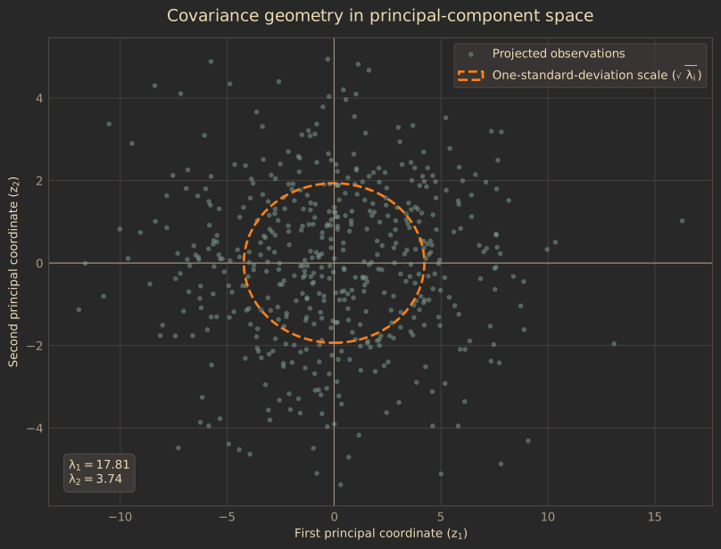
Figure 2. The first two principal-component coordinates of a six-feature dataset. The ellipse illustrates the standard-deviation scale along the principal axes.

The ellipse’s semi-axis lengths are proportional to $\sqrt{\lambda_1}$ and $\sqrt{\lambda_2}$, rather than to the eigenvalues themselves. This follows because variance is measured in squared units, whereas geometric distance is measured in the original units.

One subtlety matters here: this figure is a view of the data in principal-component coordinates, not a plot of two selected raw features. The original data have six features, even though the visualization has two axes.

6. Principal components and explained variance

Let the eigenvalues of the covariance matrix be ordered as

$$\lambda_1\geq\lambda_2\geq\cdots\geq\lambda_p\geq0.$$

The associated unit eigenvectors are $v_1,\ldots,v_p$.

The first principal component is the direction $v_1$ that maximizes projected variance. The second principal component is the direction of maximum remaining variance subject to being orthogonal to the first. Subsequent components follow the same principle.

For a covariance matrix, these directions are mutually orthogonal. The eigenvalues quantify their individual variances.

The total variance across all features is the trace of the covariance matrix:

$$\operatorname{tr}(S)=\sum_{j=1}^{p}S_{jj}.$$

Because the trace is also the sum of the eigenvalues,

$$\operatorname{tr}(S)=\sum_{j=1}^{p}\lambda_j.$$

The proportion of total variance explained by principal component $j$ is

$$\boxed{ \operatorname{EVR}_j =\frac{\lambda_j}{\sum_{k=1}^{p}\lambda_k} }.$$

The cumulative explained variance of the first $m$ components is

$$\boxed{ \operatorname{CEV}_m =\frac{\sum_{j=1}^{m}\lambda_j} {\sum_{j=1}^{p}\lambda_j} }.$$

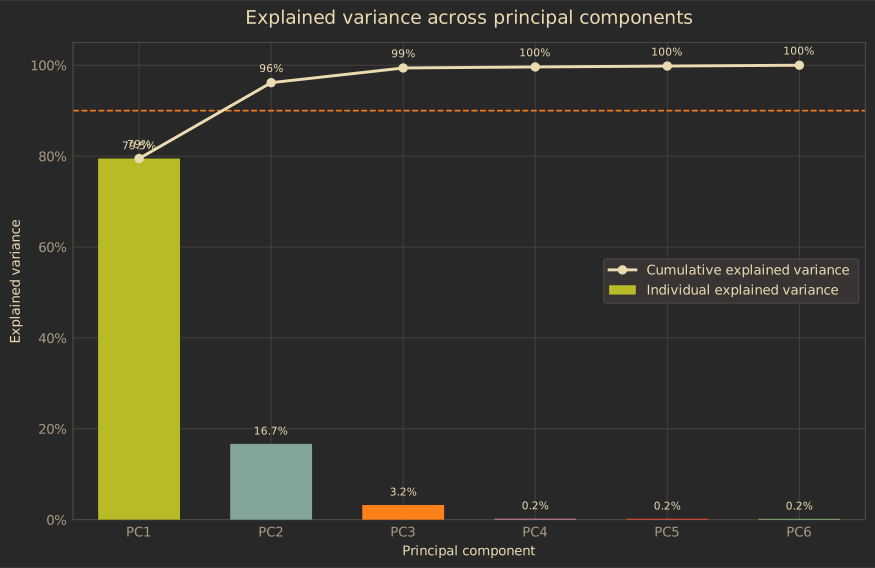
Figure 3. Individual and cumulative explained variance across the six principal components of the synthetic dataset.

The scree plot helps us assess how quickly variance accumulates as components are added. A sharp drop after the first few components can indicate that a lower-dimensional representation captures much of the dataset’s variance.

A threshold such as 90% or 95% is a useful heuristic, not a universal law. The appropriate dimensionality depends on the task, the consequences of information loss, and the downstream model.

7. A geometric view of PCA projection

After selecting the first $m$ principal components, collect their eigenvectors into the matrix

$$V_m=[v_1,\ldots,v_m].$$

The reduced representation of the centered dataset is

$$\boxed{Z_m=X_cV_m}.$$

Here, $Z_m\in\mathbb{R}^{n\times m}$: each observation is represented using $m$ coordinates rather than $p$.

We can reconstruct an approximation of the original centered data using

$$\boxed{\widehat{X}_c=Z_mV_m^\top}.$$

Substituting the expression for $Z_m$,

$$\widehat{X}_c=X_cV_mV_m^\top.$$

The matrix $V_mV_m^\top$ projects each centered observation onto the subspace spanned by the selected principal directions.

The reconstruction residual is

$$R=X_c-\widehat{X}_c.$$

This residual represents the information discarded by the reduced representation.

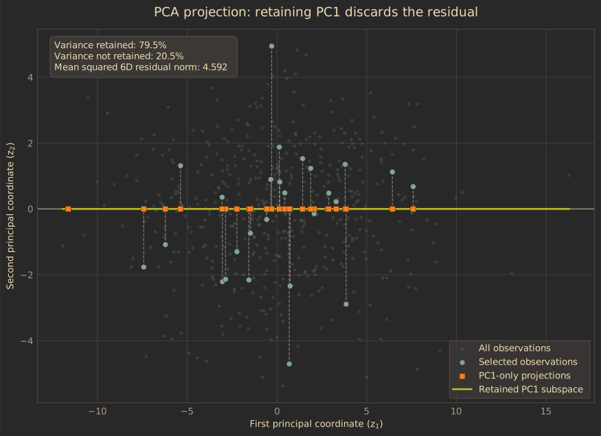
Figure 4. One-component PCA in the first two principal coordinates. Dashed segments show the visible PC2 residual for selected observations.

The visualization shows the geometry of retaining only PC1. Its horizontal coordinate is preserved, while its vertical PC2 coordinate is discarded. The reported reconstruction residual, however, is calculated in the original six-dimensional feature space and also includes the omitted components PC3 through PC6.

This distinction is important: a two-dimensional plot can help us understand a higher-dimensional projection, but it cannot display every part of a six-dimensional residual.

What does PCA optimize?

For a fixed number $m$ of components, PCA has two equivalent interpretations under the usual centered, Euclidean formulation:

1. It selects an $m$-dimensional linear subspace that maximizes the variance retained by projection.
2. It minimizes the total squared reconstruction error among rank-$m$ linear approximations of the centered data.

The second objective can be expressed as

$$\min_{\operatorname{rank}(\widehat{X}_c)\leq m} \|X_c-\widehat{X}_c\|_F^2,$$

where the Frobenius norm sums the squared errors across all entries.

This equivalence helps explain why PCA is useful for compression, visualization, and preprocessing. But it also defines its limitations: PCA preserves directions of high variance, not necessarily directions that are most predictive or most meaningful for a particular application.

8. Practical considerations: When PCA can mislead us

The mathematics is elegant, but applying PCA correctly requires attention to the data and the objective.

Feature scaling

Covariance-based PCA is sensitive to the scale of each feature. A variable measured in thousands may dominate one measured in fractions, even when their relative variation is comparable.

Standardizing features to zero mean and unit variance makes PCA equivalent to performing eigendecomposition on a correlation matrix, assuming the usual sample standardization. This is often appropriate when features use different units.

However, standardization is not automatically better. If absolute variability is meaningful, removing scale differences may discard useful information.

Outliers

Covariance depends on squared deviations from the mean. Extreme observations can therefore substantially change the covariance matrix, its eigenvalues, and its eigenvectors.

Before applying PCA, inspect distributions and outliers. Robust alternatives may be appropriate when the classical covariance estimate is not representative of the data.

Linear structure

PCA captures linear directions of variance. A dataset may lie on a curved manifold or contain clusters that cannot be represented adequately by a small number of linear components.

A high explained-variance ratio does not guarantee that all meaningful structure is preserved. Similarly, a low-dimensional projection can hide class separation or other task-relevant patterns.

Eigenvector sign and repeated eigenvalues

If $v$ is an eigenvector, then $-v$ is also an eigenvector. The sign of an individual principal component is therefore arbitrary; different implementations can return sign-flipped but mathematically equivalent components.

If eigenvalues are repeated, the individual eigenvectors within that eigenspace are not unique. The subspace remains meaningful even when a particular basis for it is not.

Sample size and rank

The centered data matrix has rank at most

$$\operatorname{rank}(X_c)\leq\min(n-1,p).$$

Consequently, if the number of features exceeds the number of observations, some covariance eigenvalues must be zero. This is a mathematical consequence of the data matrix’s rank, not necessarily a software error.

9. Eigenvalue decomposition versus singular value decomposition

We derived PCA using the eigendecomposition of the covariance matrix:

$$S=V\Lambda V^\top.$$

In practical implementations, PCA is also commonly computed using the singular value decomposition (SVD) of the centered data matrix:

$$X_c=U\Sigma V^\top.$$

The right singular vectors in $V$ are the principal directions. The covariance eigenvalues are related to the squared singular values:

$$\boxed{\lambda_j=\frac{\sigma_j^2}{n-1}}.$$

SVD provides a direct route to the principal directions without explicitly forming the covariance matrix.

Why does this matter computationally? Forming $X_c^\top X_c$ can square the condition number of the centered data matrix, potentially making numerical accuracy worse when singular values span a large range. Direct SVD is often preferable when numerical stability is important.

The trade-off is computational. Depending on the dimensions and how many components are needed, a full SVD may be unnecessarily expensive. Randomized or truncated SVD methods can be useful for large datasets when only the leading components are required.

The right choice depends on the data dimensions, available memory, required precision, and number of components. Understanding the eigendecomposition explains PCA; understanding SVD helps us implement it responsibly.

10. From a linear algebra result to a data science tool

We began with the equation

$$Av=\lambda v.$$

For a general linear transformation, this equation identifies directions that are scaled without changing their underlying line. When the matrix is a covariance matrix, the same eigenvalue equation acquires a statistical interpretation: eigenvectors identify principal directions, and eigenvalues quantify variance along them.

The chain of reasoning is direct:

1. Center the observations and construct the covariance matrix.
2. Express the variance of a projection as $w^\top Sw$.
3. Maximize that variance subject to a unit-length constraint.
4. Derive the eigenvalue equation using a Lagrange multiplier.
5. Order the eigenvectors by descending eigenvalue to obtain principal components.
6. Select a subspace and evaluate the information lost through projection.

PCA is not simply a recipe for reducing the number of columns in a dataset. It is an optimization problem with a precise objective and a clear geometric interpretation.

That is the broader lesson of eigenvectors: a useful mathematical abstraction becomes much more powerful when we understand both why it works and the assumptions under which its interpretation remains valid.